CONSISTENCY CONSTRAINTS BETWEEN CORRELATION AND CONDITIONAL DEFAULT PROBABILITIES
Category: Risk Management in Banking
From a practical standpoint, it might be easier to define simple values of conditional probabilities than specifying a correlation value between default events. For instance, assigning simple values of conditional probabilities, such as P(G| B) = 20%, is a practical way to rate support. This choice has an intuitive interpretation, since it means that the default probability of the guarantor jumps to 20% if B defaults.
The conditional probabilities of default, either P(G|B) or P(B|G), have to be within 0 and 1. Due to these constraints, the correlation p and the conditional default probabilities are subject to boundary conditions resulting from the above equations, once the standalone default probabilities of B and G are given. They serve for calculating the boundary values of p. An important practical implication is that a correlation coefficient between default events of any pair of obligors, or a conditional probability, cannot be picked up like that. Permissible values depend on the standalone default probabilities of the two obligors5. Although this is not so intuitive, it becomes obvious in certain cases. For example, if a counterparty never defaults (zero default probability), such as an Aaa guarantor, there is no correlation at all with any other risky counterparty. This implies that both the correlation and the joint default probability collapse to zero.
The next subsection makes explicit the consistency constraints between probabilities. The second one shows the relationship between the default event correlation and the conditional probabilities.
Joint Default Probabilities, Conditional Default Probability and Correlation
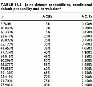
Table 41.5 calculates the joint default probabilities when the default correlation and the corresponding conditional default probability of the guarantor given Bs default vary. The table also illustrates the existence of boundary values of P(G|B) and P(G, B). These values are such that the conditional probability or the default correlation cannot take unacceptable values outside the allowed ranges, 0 to 1 for conditional probability and —1 to +1 for default correlation.
Credit Risk Valuation and
Credit Spreads
Credit risk events, defaults and migrations, result in changes in value of facilities. Between now and the horizon, defaults and migrations are random, so that there is a distribution of the future values at a given horizon over the entire spectrum of risk migrations. This distribution of values at a given horizon serves to determine the potential losses, and the loss statistics and loss percentiles measuring credit risk Value at Risk (VaR). For default-only models, the distribution of values for each facility collapses to two states, default and non-default. For full valuation models, migrations to a different risk class than the original result in changes in values because the risk changes. The most prominent models, KMV Portfolio Manager, Credit Metrics and Credit Portfolio View (CPV) are full economic valuation models. CreditRisk+ is a default model.
Credit risk models value credit risk only, considering that other risks, market risk and interest rate risk, are taken care of by other tools. They use a mark-to-model technique, restricting the mark-to-market of assets to migrations of credit risk only. Valuation at horizon uses the credit spreads of various risk classes for discounting contractual cash flows, or, alternatively, expected cash flows that are lower because of default probabilities. This is a future valuation, or mark-to-future, using the entire spectrum of possible credit states at a future time point.
Beyond risk measuring, credit risk valuation serves two other purposes:
• Valuation of traded and non-traded assets in a manner consistent with the market valuation of credit risk.
• Modelling the implied default probabilities in bond prices, as risk-neutral probabilities. The technique makes explicit the relation between spreads, risk-neutral probabilities, rather than natural probabilities, and recovery rates.
The valuation of risky debt uses either one of two equivalent techniques:
• Discounting contractual cash flows using risky yields, risk-free yields plus credit spreads;
• Discounting expected cash flows at the risk-free rates using the risk-neutral probabilities for calculating the expected values of cash flows.
Under risk aversion, the probabilities required to calculate the expected flows are risk-neutral probabilities. Risk-neutral probabilities differ from natural probabilities because they embed the risk aversion of the market. Arbitrage arguments demonstrate that the above two techniques are equivalent. Therefore, credit spreads relate to risk-neutral probabilities and recovery rates.
Valuation is a key building block for determining the value distribution at a forward horizon. In risk models, valuation is forward, at the horizon, for all possible credit risk scenarios, in order to derive a distribution of future values. Matrix valuation refers to the usage of credit spreads for valuing any asset at some horizon, using the array of credit states. The technique combines transition probabilities with the credit spreads corresponding to the final credit states. Most portfolio models use the matrix technique. Implementing the risk-neutral valuation for a future date is more challenging because of the need to have risk-neutral probabilities. Only KMV Portfolio Manager provides risk-neutral valuation as an alternative option to matrix valuation.
The first section defines credit spreads and shows how to derive them from the spot and forward risk-free and risky yield curves. The second section describes the two basic techniques for valuation. The third section discusses the relation between valuation, credit risk and maturity. The last section describes the valuation building blocks of different credit risk models. The appendix to this chapter further details some counterintuitive effects of this mechanism.
CREDIT SPREADS
The market provides yield curves, for the risk-free yields of government debt and for risky debts of all ratings. Standard practices derive risky yields by grouping bonds according to their ratings. Credit spreads are differences between the risky yields and the risk-free yields. This section discusses credit spreads, both spot and forward, from such market yields.
Calculation of Credit Spreads
The calculation of spreads results from spot and forward risky and risk-free yield curves. When using the spot rates, we obtain spot credit spreads. When using the forward yield curves, we obtain forward credit spreads.
Calculation of Spot Spreads
A credit spread is the difference between the yield of a risky debt and the risk-free rate between any two dates. Formally, if y and yf are the risky yield and the risk-free yield:
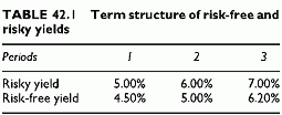
The calculation is similar for spot credit spreads and forward credit spreads. Using the yields of the risk-free and of the risky debts, spot credit spreads are 0.50% for 1 year, 1% for 2 years and 1.8% for 3 years (Table 42.1).


