CREDIT METRICS CORRELATED JOINT MIGRATION MATRICES
Category: Risk Management in Banking
Credit Metrics develops a technique to find the distribution of values of a portfolio at a future time point from transition matrices. The technique requires using correlated transition probabilities for each pair of obligors. Correlated migration probabilities result from the correlations of unobservable asset values. They make it possible to describe all possible credit states for each pair of obligors in a squared matrix called a joint migration matrix. The joint migration matrix shows, for each pair of firms, initially in risk classes i and j, the probabilities of ending in the risk classes k and l, with i, j, k and l being classes of the same rating scale. A transition matrix shows all future states of a single obligor at the horizon. A joint migration matrix shows the joint migration probabilities of any pair of credit states of any pair of obligors. These joint migration probabilities depend on the correlation between the obligors risks. Details follow with a simplified example.
Credit Metrics Approach
Should the transitions be independent for each obligor, the joint migration probability for any pair of states would be the product of the probabilities of independent migration probabilities. However, the joint migration probabilities differ from this value because of correlations. When economic conditions worsen, chances are that default probabilities increase, and that all downward migrations increase, and they correlate. This is also the principle underlying the CPV view of modelled migrations. This makes it necessary to use correlated joint migration matrices instead of unconditional migrations.
For each initial credit state, we know the unconditional probabilities of moving to other credit states. For instance, the standard transition matrix could tell us that the probability of X moving from A to B is 5% and Y moving from B to C is 4%. If the transitions of firms X and Y are independent, the probability that the pair of obligors moves to the pair of risk classes B and C would be 5% x 4% = 0.2%. From the examples of matrices below, we find that the probability of ending in this state is in fact 0.2%, higher than the product. The reason is that migrations tend to correlate so that the joint migration probability embeds a correlation.
The technique for correlating migrations is to use the correlation between asset values of firms to determine the probability of the pair falling into any combination of two rating classes. To illustrate the process, we use conditional probabilities, which allow us to make explicit all details of the calculations. With zero correlations, the conditional probabilities are equal to the unconditional ones. With positive correlations, they are higher. In the example below, we make explicit the differences between the independent and the correlated case using conditional probabilities to calculate directly the joint probabilities instead of asset value correlations.
Unconditional Migration Matrix
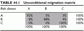
The starting point is the unconditional migration matrix. In this matrix, the default state is C. It is the absorbing state. Once there, there is no way out. All probabilities sum to 100% across rows and across columns (Table 44.1)
In order to find the state of a pair of obligors, X and Y, we need to select the initial state of each obligor. We assume that X is in state A and that Y is in state B. The next subsection examines the case of X remaining in state A, while Y migrates upwards from its initial state B to the state A. Due to migrations, the final states follow the migration matrix. We show what happens in the case of independence and of correlated migrations.
Independent Migrations
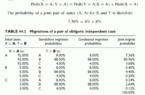
For example, the first line of Table 44.2 indicates that: the standalone migration probability of X staying in A is 92%; the standalone probability that Y migrates from B to A is 8%; the conditional probability that Y moves from B to A given that X stays in A is 8%. The latter conditional probability, 8%, is equal to the unconditional migration probability that Y migrates from B to A because this migration is assumed, in this table, independent of what happens to X. The general law of conditional probability states that:
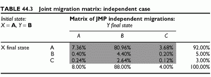
This probability appears in the last column and is the joint migration probability of the pair of states (A, B) to (A, A), where the first state refers to X and the second to Y. As usual with independent events, this is simply the product of the unconditional migration probabilities. It is convenient to group all such joint migration probabilities (JMP) in a matrix, shown in Table 44.3, where each cell provides the joint probability of all nine possible pairs of final states.
The benefit of using the above conditional probability formula becomes clearer when we use conditional migration probabilities that differ from the unconditional ones, in order to capture correlations between migrations. The next subsection shows how figures change in the interdependent case.
Correlated Migrations
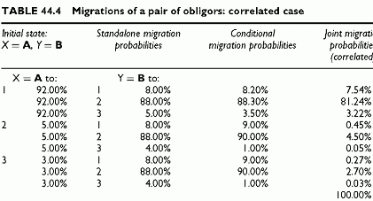
In order to control the joint migrations, we use conditional probabilities different from the standalone probabilities. In Table 44.4, the columns showing the conditional probabilities and the resulting joint migration probabilities change. The correlation between migration events implied in the joint migration probability results from the formula relating this correlation with unconditional and joint migration probabilities. There is no need to calculate them here, and we focus on the structure of the matrices.
The values refer to the final state. The calculation is: Prob(X = A, Y = A) = 8% x 8.20% = 7.54%. This joint migration is higher than the previous 7.36% value due to correlations. Note that this is not the case for all joint migration probabilities. When the conditional probabilities are above the standalone probabilities the resulting joint migration probability is above that of the independent case, and conversely. If this were the case for all states, all probabilities would sum to more than 1, which is impossible. Increasing some migration probabilities implies that others decrease. All joint migration probabilities are equal to the product of the unconditional probabilities. Their sum is 100%. This effect appears in Table 44.4 and in the new matrix of pairs of final states (Table 44.5).


